4.2. Optimization on a closed system: creation of a target evolution operator

This tutorial demonstrates a basic optimization performed on a simple three-level quantum model of the Nitrogen-vancancy center in diamond. The goal, in this case, is to find a pulse that induces a given evolution operator (a gate, in the language of quantum information theory).

The model is defined by the three-level Hamiltonian: \begin{align} H(u, t) &= H_0 + V(u, t), \\ H_0 &= -B_s S_z + N_z S_z^2 + N_{xy}(S_x^2-S_y^2), \\ V(u, t) &= - g_x(u, t) B_d S_x - g_y(u, t) B_d S_y. \end{align} This model is taken from [Ikeda et al, Science Advances 6, eabb4019 (2020)]. \(S_x, S_y\) and \(S_z\) are the spin operators, whereas \(N_z\), \(N_{xy}\), \(B_s\), and \(B_d\) are constants. The shape of the real time-dependent control functions \(g_x\) and \(g_y\) is explained below.

import numpy as np
import matplotlib
from copy import deepcopy
import matplotlib.pyplot as plt
import qutip as qt

import qocttools
import qocttools.hamiltonians as hamiltonians
import qocttools.target as target
import qocttools.pulses as pulses
import qocttools.qoct as qoct
import qocttools.solvers as solvers

It is good practice to print the precise version of the software that you are using.

qocttools.about()

No git dir found

Running qocttools version 0.0.14

data = []

Now, we build the static Hamiltonian \(H_0\) (stored into the Qobj object H0), and the two coupling operators \(V_1 = -B_d S_x\) and \(V_2 = -B_d S_y\) (stored into the Qobj objects V[0] and V[1]). The function system_definition in principle returns some Lindblad operators, but those are not used in this tutorial. The field-free eigenvalues are stored stored in the array e and the eigenfunctions in psi.

Sx = qt.jmat(1, "x")
Sy = qt.jmat(1, "y")
Sz = qt.jmat(1, "z")
Bs = 0.3
Nz = 1.00
Nxy = 0.05
Bd = 0.1
omega = 1.00
# We assume in this tutorial that the dissipation is zero.
# gamma = 0.2
gamma = 0.0
beta = 3.0
d = 3
dim = d**2

def system_definition():
    H0 = -Bs * Sz + Nz * Sz**2 + Nxy * (Sx**2 - Sy**2)
    Vx = -Bd * Sx
    Vy = -Bd * Sy
    A = []
    e, psi = H0.eigenstates()
    for i in range(d):
        for j in range(d):
            if j == i:
                continue
            gammaij = gamma * np.exp(-beta*e[j]) / (np.exp(-beta*e[i])+np.exp(-beta*e[j]))
            A.append( np.sqrt(gammaij) * psi[j] * psi[i].dag())
    return H0, [Vx, Vy], A, e, psi

H0, V, A, e, psi = system_definition()

print("Field-free eigenvalues = {}".format(e))

Field-free eigenvalues = [0.         0.69586187 1.30413813]

The first step is to create the an object of hamiltonian class:

H = hamiltonians.hamiltonian(H0, V)

The energy and time scales of the system are determined by the natural frequencies, which are the eigenenergy differences. We will use the difference between the ground and the first excited state to define a characteristic system frequency omega, that we will use as a reference for the rest of the definitions. tau will be the corresponding period.

omega = e[1]-e[0]
tau = 2.0*np.pi/omega

Now we consider the total propagation time. To make the process easier, it is useful to make sure that the total propagation time includes several times the characteristic period tau. In this case, we will make it ten times larger. This also defines a fundamental frequency, \(\omega_0 = 2\pi/T\).

T = 5 * tau
omega0 = 2.0*np.pi/T
print("omega0 = {:.4f}".format(omega0))

omega0 = 0.1392

Now we create the Target object. In this case, it is an “evolutionoperator” type, since what we want to do is to find a pulse that induces a given evolution operator. For this example, we choose a three-level “gate” that is a rotation gate (a member of \(SU(3)\)), built by taking ane exponential of the first Gell-Mann matrix (The Gell-Mann matrices are a set of eight linearly independent 3x3 traceless Hermitian matrices. They span the Lie algebra of the SU(3) group in the defining representation. They are the equivalent of the Pauli matrices, for three-dimensional problems).

lambda1 = qt.Qobj( np.array([[0, 1, 0], [1, 0, 0], [0, 0, 0]]) )
R = ((-1j * (np.pi/2) ) * lambda1).expm()

tg = target.Target("evolutionoperator", Utarget = R)

Now, we must create the pulse objects, i.e. the control functions. In this case, we have two perturbation operators, and we need two control functions. In this example, we will choose a Fourier-series parametrization for both control functions.

A Fourier series must be cutoff at some maximum frequency \(M\omega_0\). We will set \(M=15\), which ensures that the relevant frequency \(\omega\) is lower than the maximum frequency. Then we must give initial-guess values to the amplitudes of the Fourier series (which are the control parameters). There are \(2M+1\) parameteres in each Fourier series (\(M\) for the cosines, \(M\) for the sines, and 1 for the zero-frequency term). We will simply set some of the parameters to some \(\kappa\) value, and zero for the rest of them.

A better alternative would be to use random values, but in order to make sure that the tutorial always produces the same result, we will not use that option here.

M = 15
kappa = 0.1

u1 = np.zeros(2*M+1)
u2 = np.zeros(2*M+1)
u1[3] = kappa
u2[4] = kappa

# The following code sets random numbers for the control parameters
#a = -bound
#b = bound
#u1 = (b-a) * np.random.rand(2*M+1) + a
#u2 = (b-a) * np.random.rand(2*M+1) + a

We place the pulse objects into a list f.

f = []
f.append(pulses.pulse("fourier", T, u = u1))
f.append(pulses.pulse("fourier", T, u = u2))
f0 = deepcopy(f)

u0 will hold all the control parameters (the parameters of all the pulses together).

u0 = pulses.pulse_collection_get_parameters(f)

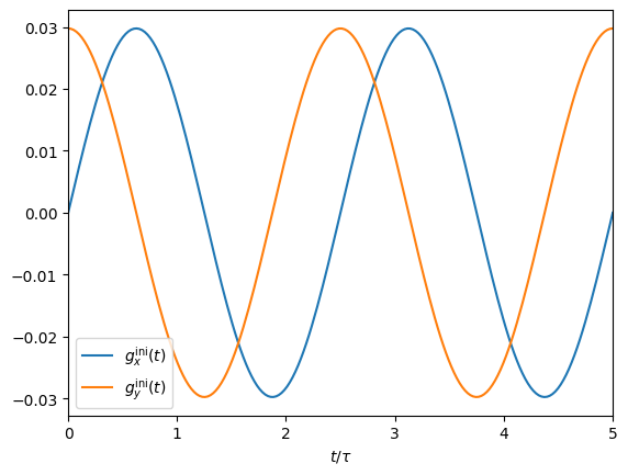
Let us plot to see how the pulses look like.

fig, ax = plt.subplots()

ts = np.linspace(0, T, 200)
ax.plot(ts/tau, f0[0].fu(ts), label = r"$g_x^{\rm ini}(t)$")
ax.plot(ts/tau, f0[1].fu(ts), label = r"$g_y^{\rm ini}(t)$")
ax.set_xlabel(r"$t/\tau$")
ax.set_xlim(0, T/tau)
ax.legend()

plt.show()

We now build the main object, of class Qoct. Along with the Hamiltonian H, the target tg, and the set of control functions f, we need to pass the initial state, which in this case it has to be the identity matrix (the evolution operator at time zero). Also, ntsteps, which is the number of time steps used to discretize the time interval for the numerical integration. The higher, the more precise the calculations will be, but they will also be slower.

ntsteps = 200
U0 = qt.qeye(d)
opt = qoct.Qoct(H, T, ntsteps, tg, f, U0)

Let us see what the initial pulse does: we will propagate the system using the initial guess pulses, and we will plot the value of the target function as it evolves in time:

\begin{equation} F(t) = \frac{1}{d^2} \vert R \cdot U(t)\vert^2 \end{equation}

where the dot product is the Fröbenius inner product.

In order to the system propagation, we will use the solve() function and, in this case, the cfmagnus4 method (see the documentation of the solve() function to learn about the propagation methods used by qocttools).

ts = np.linspace(0, T, ntsteps)
res = solvers.solve('cfmagnus4', H, f, U0, ts)
Ft = np.zeros(ntsteps)
for j in range(ntsteps):
    Ft[j] = (1/d**2) * np.abs((R.dag() * res[j]).tr())**2

fig, ax = plt.subplots()
ax.plot(ts/tau, Ft, label = r"$F(U(t))$")
ax.set_xlabel(r"$t/tau$")
ax.set_xlim(0, T/tau)
ax.legend()
plt.show()

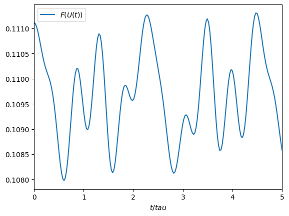
As one can see, the value of the plotted function remains close to 0.1 all the time when using the initial guess (the value of the function is one when the evolution operator is equal – or equivalent – to the target operator \(R\)).

Before launching the optimization, let us check that the gradient is computed correctly. We can use for that purpose the check_grad() method of the Qoct class. It computes the gradient using the QOCT formula, and using finite differences. Both numbers should match if everything is OK.

derqoct, dernum, error, elapsed_time = opt.check_grad(u0)
print(derqoct, dernum, error)

0.15383541010075516 0.15383511158066712 1.0796918914479647e-14

Finally, we launch the maximization calculation, using the maximize() method.

x, optval, result = opt.maximize(maxeval = 100,
                                 stopval = 0.99,
                                 verbose = True)
data.append(optval)

0 0.108575 (0.069700 s)
1 0.156977 (0.087020 s)
2 0.060585 (0.086820 s)
3 0.728001 (0.072904 s)
4 0.827513 (0.087359 s)
5 0.871092 (0.073293 s)
6 0.875651 (0.086773 s)
7 0.878619 (0.069639 s)
8 0.889817 (0.088577 s)
9 0.902860 (0.086685 s)
10 0.925295 (0.073400 s)
11 0.962166 (0.087162 s)
12 0.968960 (0.087776 s)
13 0.970434 (0.087238 s)
14 0.988589 (0.082098 s)
15 0.999418 (0.086732 s)
Successfull termination with result code = 2
("Stop value reached")

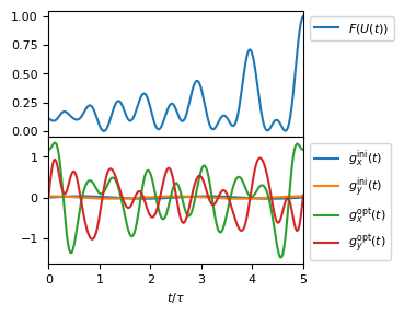
As you can see, the optimization proceeds pretty fast towards the optimal value. Let us see the behaiour of the target function in a plot.

ts = np.linspace(0, T, ntsteps)
res = solvers.solve('cfmagnus4', H, f, U0, ts)
Ft = np.zeros(ntsteps)
for j in range(ntsteps):
    Ft[j] = (1/d**2) * np.abs((R.dag() * res[j]).tr())**2

Finally, we can look at how the target function evolves in time until it reaches a value close to the ideal maximum on one, and we compare now in a plot the initial guess versus the optimized pulse.

plt.rcParams["font.size"] = "8"
plt.rcParams["figure.autolayout"] = False

fig, ax = plt.subplots(2, 1, figsize=(3, 3), sharex = True)
fig.subplots_adjust(hspace=0)

ax[0].plot(ts/tau, Ft, label = r"$F(U(t))$")
#ax[0].set_xlabel(r"$t/\tau$")
ax[0].set_xlim(0, T/tau)
#ax[0].label_outer()
ax[0].legend(bbox_to_anchor = (1.0, 1.0), loc = 'upper left')

#fig, ax = plt.subplots(2, figsize=(3,2))

ts = np.linspace(0, T, 200)

ax[1].plot(ts/tau, f0[0].fu(ts), label = r"$g_x^{\rm ini}(t)$")
ax[1].plot(ts/tau, f0[1].fu(ts), label = r"$g_y^{\rm ini}(t)$")
ax[1].plot(ts/tau, f[0].fu(ts), label = r"$g_x^{\rm opt}(t)$")
ax[1].plot(ts/tau, f[1].fu(ts), label = r"$g_y^{\rm opt}(t)$")
ax[1].set_xlabel(r"$t/\tau$")
ax[1].set_xlim(0, T/tau)
#ax[1].label_outer()
ax[1].legend(bbox_to_anchor = (1.0, 1.0), loc = 'upper left')

fig.savefig("closed-gate.pdf", bbox_inches = 'tight')
plt.show()

# This file is used by the testing script of the code.
with open("data", "w") as f:
    for i in data:
        f.write("{:.14e}\n".format(i))