4.1. Optimization on a closed system

This tutorial demonstrates a basic optimization on a simple three-level quantum model of the Nitrogen-vancancy center in diamond. The goal is to find a pulse that drives the system from its ground to its highest energy state.

The model is defined by the three-level Hamiltonian:

\begin{align} H(u, t) &= H_0 + V(u, t), \\ H_0 &= -B_s S_z + N_z S_z^2 + N_{xy}(S_x^2-S_y^2), \\ V(u, t) &= - g_x(u, t) B_d S_x - g_y(u, t) B_d S_y. \end{align}

This model is taken from [Ikeda et al, Science Advances 6, eabb4019 (2020)]. \(S_x, S_y\) and \(S_z\) are the spin operators, whereas \(N_z\), \(N_{xy}\), \(B_s\), and \(B_d\) are constants. The shape of the real time-dependent control functions \(g_x\) and \(g_y\) is explained below.

import numpy as np
import matplotlib
from copy import deepcopy
import matplotlib.pyplot as plt
import qutip as qt

import qocttools
import qocttools.hamiltonians as hamiltonians
import qocttools.target as target
import qocttools.pulses as pulses
import qocttools.qoct as qoct
import qocttools.solvers as solvers

It is good practice to print the precise version of the software that you are using.

qocttools.about()

No git dir found

Running qocttools version 0.0.14

data = []

Now, we build the static Hamiltonian \(H_0\) (stored into the Qobj object H0), and the two coupling operators \(V_1 = -B_d S_x\) and \(V_2 = -B_d S_y\) (stored into the Qobj objects V[0] and V[1]). The function system_definition in principle returns some Lindblad operators, but those are not used in this tutorial. The field-free eigenvalues are stored stored in the array e and the eigenfunctions in psi.

Sx = qt.jmat(1, "x")
Sy = qt.jmat(1, "y")
Sz = qt.jmat(1, "z")
Bs = 0.3
Nz = 1.00
Nxy = 0.05
Bd = 0.1
omega = 1.00
# We assume in this tutorial that the dissipation is zero.
# gamma = 0.2
gamma = 0.0
beta = 3.0
d = 3
dim = d**2

def system_definition():
    H0 = -Bs * Sz + Nz * Sz**2 + Nxy * (Sx**2 - Sy**2)
    Vx = -Bd * Sx
    Vy = -Bd * Sy
    A = []
    e, psi = H0.eigenstates()
    for i in range(d):
        for j in range(d):
            if j == i:
                continue
            gammaij = gamma * np.exp(-beta*e[j]) / (np.exp(-beta*e[i])+np.exp(-beta*e[j]))
            A.append( np.sqrt(gammaij) * psi[j] * psi[i].dag())
    return H0, [Vx, Vy], A, e, psi

H0, V, A, e, psi = system_definition()

print("Field-free eigenvalues = {}".format(e))

Field-free eigenvalues = [0.         0.69586187 1.30413813]

The first step is to create the an object of hamiltonian class.

H = hamiltonians.hamiltonian(H0, V)

The objective is for the system to transition from the ground state to the first excited state. Therfore, we will define a relevant frequency omega, given by the energy difference between those states. The relevant period is the one corresponding to that frequency

omega = e[1]-e[0]
tau = 2.0*np.pi/omega

Now we consider the total propagation time. To make the transition easier, it is useful to make sure that the total propagation time includes several time the relevant period tau. In this case, we will make it ten times larger.

The definition of a propagation time \(T\) also defines a “fundamental frequency”, \(\omega_0 = 2\pi/T\).

T = 3 * tau
omega0 = 2.0*np.pi/T
print("omega0 = {:.4f}".format(omega0))

omega0 = 0.2320

Now we create the Target object. In this case, it is an “expectationvalue” type, since what we want to do is to maximize the expectation value of \(O = \vert\phi_1\rangle \langle\phi_1\vert\), i.e. the population of the first excited state. See the documenation of the Target class to learn about other options that can be used.

O = psi[1] * psi[1].dag()
tg = target.Target("expectationvalue", operator = O)

Thus, we are defining the target function as: \begin{equation} F(\psi, u) = \langle \psi \vert O \vert \psi \rangle\,, \end{equation} so that the function of the control parameters \(u\) that is to be optimized is: \begin{equation} G(u) = F(\psi_u(T), u)\,. \end{equation}

Now, we must create the pulse objects, i.e. the control functions. In this case, we have two perturbation operators, and we need two control functions. In this example, we will choose a Fourier-series parametrization for both control functions.

A Fourier series must be cutoff at some maximum frequency \(M\omega_0\). We will set \(M=15\), which ensures that the relevant frequency \(\omega\) is lower than the maximum frequency. Then we must give initial-guess values to the amplitudes of the Fourier series (which are the control parameters). There are \(2M+1\) parameteres in each Fourier series (\(M\) for the cosines, \(M\) for the sines, and 1 for the zero-frequency term). We will simply set some of the parameters to some \(\kappa\) value, and zero for the rest of them.

A better alternative would be to use random values, but in order to make sure that the tutorial always produces the same result, we will not use that option here.

M = 10
kappa = 1.0

u1 = np.zeros(2*M+1)
u2 = np.zeros(2*M+1)
u1[3] = kappa
u1[5] = kappa
u2[5] = kappa
u2[4] = kappa


# The following code sets random numbers for the control parameters
#bound = kappa
#a = -bound
#b = bound
#u1 = (b-a) * np.random.rand(2*M+1) + a
#u2 = (b-a) * np.random.rand(2*M+1) + a

We place the pulse objects into a list f.

f = []
f.append(pulses.pulse("fourier", T, u = u1))
f.append(pulses.pulse("fourier", T, u = u2))
f0 = deepcopy(f)

u0 will hold all the control parameters (the parameters of all the pulses together).

u0 = pulses.pulse_collection_get_parameters(f)

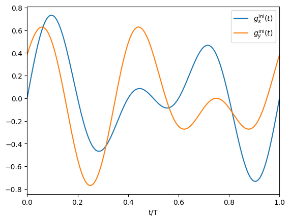
Let us plot to see how the pulses look like.

fig, ax = plt.subplots()

ts = np.linspace(0, T, 200)
ax.plot(ts/T, f0[0].fu(ts), label = r"$g_x^{\rm ini}(t)$")
ax.plot(ts/T, f0[1].fu(ts), label = r"$g_y^{\rm ini}(t)$")
ax.set_xlabel("t/T")
ax.set_xlim(0, 1)
ax.legend()

plt.show()

We now build the main object, of class Qoct. Along with the Hamiltonian H, the target tg, and the set of control functions f, we need to pass the initial state, in our case the ground states psi[0]. Also, ntsteps, which is the number of time steps used to discretize the time interval for the numerical integrations of the equations that need to be solved. The higher, the more precise the calculations will be, but they will also be slower.

ntsteps = 400
opt = qoct.Qoct(H, T, ntsteps, tg, f, psi[0])

Let us see what the initial pulse does: we will propagate the system using the initial guess pulses, and we will plot the populations of each state as a function of time.

In order to the system propagation, we will use the solve() function and, in this case, the cfmagnus4 method (see the documentation of the solve() function to learn about the propagation methods used by qocttools).

ts = np.linspace(0, T, ntsteps)
res = solvers.solve('cfmagnus4', H, f, psi[0], ts)
ps = np.zeros([ntsteps, d])
for k in range(d):
    for j in range(ntsteps):
        ps[j, k] = qt.expect(psi[k]*psi[k].dag(), res[j])

fig, ax = plt.subplots()
ax.plot(ts, ps[:, 0], label = r"$P_0$")
ax.plot(ts, ps[:, 1], label = r"$P_1$")
ax.plot(ts, ps[:, 2], label = r"$P_2$")
ax.set_xlabel("t")
ax.set_xlim(0, T)
ax.legend()
plt.show()

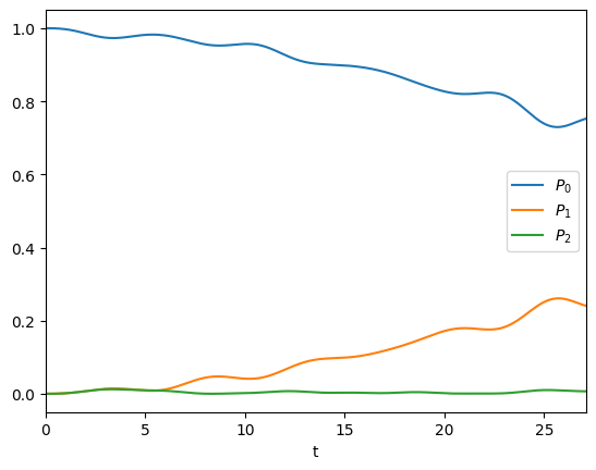
As one can see, it does nothing: the populations of the excited state remain close to zero, and the population of the initial ground state remains close to one. This can be checked by computing the value of the target function for this initial guess pulse, which can be done simply by using the gfunc method:

print("G(u0) = {}".format(opt.gfunc(u0)))

G(u0) = 0.24081398319554317

We want to change that, and force a population transfer to the first excited state.

Before launching the optimization, let us check that the gradient is computed correctly. We can use for that purpose the check_grad() method of the Qoct class. It computes the gradient using the QOCT formula, and using finite differences. Both numbers should match if everything is OK.

derqoct, dernum, error, elapsed_time = opt.check_grad(u0)
print(derqoct, dernum, error)

0.25513488901671894 0.2551348688953757 2.8993474288085963e-13

Finally, we launch the maximization calculation, using the maximize() method. Here, we will set a maximum number of evaluations through the maxeval argument, a stop value to stop the iterations in case a certain threshold is reached through the stopvalargument, and we will set verbose to True so that we can see the optimization process as it runs.

pulses.pulse_collection_set_parameters(f, u0)
x, optval, result = opt.maximize(maxeval = 100,
                                 stopval = 0.99,
                                 verbose = True,
                                 upper_bounds = 2*kappa * np.ones_like(u0),
                                 lower_bounds = -2*kappa * np.ones_like(u0))

0 0.240814 (0.142161 s)
1 0.454806 (0.121425 s)
2 0.967806 (0.142146 s)
3 0.978757 (0.131680 s)
4 0.999168 (0.140300 s)
Successfull termination with result code = 2
("Stop value reached")

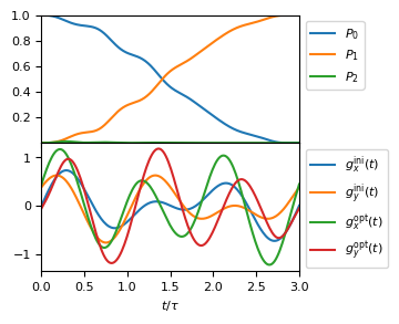
As you can see, the optimization proceeds pretty fast towards the optimal value, achieving full population of the target excited state. Let us see this transfer in a plot.

ts = np.linspace(0, T, ntsteps)
res = solvers.solve('cfmagnus4', H, f, psi[0], ts)
ps = np.zeros([ntsteps, d])
for k in range(d):
    for j in range(ntsteps):
        ps[j, k] = qt.expect(psi[k]*psi[k].dag(), res[j])

We now plot the results: in the top plot, the populations of the states as they evolve in time; in the bottom plot, the initial and optimized pulses.

plt.rcParams["font.size"] = "8"
plt.rcParams["figure.autolayout"] = False

fig, ax = plt.subplots(2, 1, figsize=(3, 3), sharex = True)
fig.subplots_adjust(hspace=0)

ax[0].plot(ts/tau, ps[:, 0], label = r"$P_0$")
ax[0].plot(ts/tau, ps[:, 1], label = r"$P_1$")
ax[0].plot(ts/tau, ps[:, 2], label = r"$P_2$")
#ax.set_xlabel(r"$t/\tau$")
ax[0].set_xlim(0, T/tau)
ax[0].set_ylim(0, 1)
ax[0].set_yticks([0.2, 0.4, 0.6, 0.8, 1.0])
ax[0].legend(bbox_to_anchor = (1.0, 1.0), loc = 'upper left')

ts = np.linspace(0, T, 200)

ax[1].plot(ts/tau, f0[0].fu(ts), label = r"$g_x^{\rm ini}(t)$")
ax[1].plot(ts/tau, f0[1].fu(ts), label = r"$g_y^{\rm ini}(t)$")
ax[1].plot(ts/tau, f[0].fu(ts), label = r"$g_x^{\rm opt}(t)$")
ax[1].plot(ts/tau, f[1].fu(ts), label = r"$g_y^{\rm opt}(t)$")
ax[1].set_xlabel(r"$t/\tau$")
ax[1].set_xlim(0, T/tau)
ax[1].legend(bbox_to_anchor = (1.0, 1.0), loc = 'upper left')

fig.savefig("closed.pdf", bbox_inches = 'tight')
plt.show()

4.1.1. Calculations using the “generic” target type

Finally, let us repeat the very same calculations, but using the “generic” option for defining the target objetc. In this way, one can define any target function in the form: \begin{equation} F = F(\psi, u)\,, \end{equation} where \(\psi\) is the wave function at the end of the propagation (since, for this kind of calculations, qocttools only performs terminal-like optimal control in the current version). In addition, \(F\) may depend on the set of parameters \(u\) of the control functions (in order to allow for the presence of penalties, etc. Often, this explicit dependency is absent, but the function interface must allow it).

In addition, one must define the derivative of this function, \(\frac{\delta F}{\delta \psi^*}\).

Thus, for example, for the simple case that we are dealing with: \begin{equation} F(\psi, u) = \langle \psi \vert O \vert \psi \rangle\,, \end{equation} and \begin{equation} \frac{\delta F}{\delta \psi^*} = O \vert \psi\rangle\,. \end{equation} These functions can be coded as:

def Fpsi(psi, u):
    return qt.expect(O, psi)
def dFdpsi(psi, u):
    return O * psi

If there were an explicit dependence on \(u\), we would also have to define a function \(\frac{\partial F}{\partial u}\), to be passed to the dFdu argument of the Target class constructor.

Then, we can define the Target object as:

tg = target.Target("generic", Fyu = Fpsi, dFdy = dFdpsi)

opt = qoct.Qoct(H, T, ntsteps, tg, f, psi[0])

pulses.pulse_collection_set_parameters(f, u0)

derqoct, dernum, error, elapsed_time = opt.check_grad(u0)
print(derqoct, dernum, error)

0.25513488901671894 0.2551348688953757 2.8993474288085963e-13

pulses.pulse_collection_set_parameters(f, u0)
x, optval, result = opt.maximize(maxeval = 100,
                                 stopval = 0.99,
                                 verbose = True,
                                 upper_bounds = 2*kappa * np.ones_like(u0),
                                 lower_bounds = -2*kappa * np.ones_like(u0))
data.append(optval)

0 0.240814 (0.143129 s)
1 0.454806 (0.132758 s)
2 0.967806 (0.140912 s)
3 0.978757 (0.128799 s)
4 0.999168 (0.142013 s)
Successfull termination with result code = 2
("Stop value reached")

Of course, it does not make sense to use this “generic” mode to do the same calculation than we did before. However, it can be used to define any target function

4.1.2. Calculations using automatic differentiation

(WARNING: THE SUPPORT FOR AUTOMATIC DIFFERENTIATION IS STILL IN DEVELOPMENT, AND THEREFORE IT IS PROBABLY VERY UNSTABLE)

In some circumstances, one may want to use a target definition whose derivative with respect to the wave function (or the density matrix, or the evolution operator) is not easy to write as a Python function, or is not known, etc. In that case, one may use automatic differentiation and skip the specification of the dFdy function. For that purpose, qocttools is using the jax library, that should be loaded with:

import jax; jax.config.update('jax_platform_name', 'cpu')
import jax.numpy as jnp

(The specification of cpu instead of gpu can probably be lifted if you can use GPUs, but I have not tested that)

We do have to define the function \(F\) to pass it to the Fyu argument of the Target object constructor. The key point is that this function no longer works with qutip objects, but it should work with jax.numpy objects, and do the calculations using those. Thus, for example, to replicate the calculations above:

def Fpsi(psi, u):
    return jnp.vdot(psi, jnp.matmul(O.full(), psi)).real

Then, when building the Target object, the dFdy argument should be given the string ‘ad’ as value.

tg = target.Target("generic", Fyu = Fpsi, dFdy = 'ad')

The rest is the same:

opt = qoct.Qoct(H, T, ntsteps, tg, f, psi[0])

pulses.pulse_collection_set_parameters(f, u0)
x_ad, optval, result = opt.maximize(maxeval = 100,
                                 stopval = 0.99,
                                 verbose = True,
                                 upper_bounds = 2*kappa * np.ones_like(u0),
                                 lower_bounds = -2*kappa * np.ones_like(u0))
data.append(optval)

0 0.240814 (0.462121 s)
1 0.454806 (0.129268 s)
2 0.967805 (0.136348 s)
3 0.978757 (0.116518 s)
4 0.999168 (0.128457 s)
Successfull termination with result code = 2
("Stop value reached")

In this case, the calculations are different; the slight numerical differences that one gets when computing the derivative with AD with respect to using the analytical formula seem to lead to a different convergence history. But the final optimal solution is very similar, as it can be checked computing the norm of the difference:

print("||x|| = {}, ||x_ad|| = {}".format(np.linalg.norm(x), np.linalg.norm(x_ad)))
print("||x-x_ad|| / ||x|| = {}".format(np.linalg.norm(x-x_ad)/np.linalg.norm(x)))

||x|| = 3.5061442275206742, ||x_ad|| = 3.5061442205780224
||x-x_ad|| / ||x|| = 3.8825570409529546e-08

It should be stressed that automatic differentiation is used to obtain the derivative \begin{equation} \frac{\delta F}{\delta \psi^*} \end{equation} that is used to build the finite-value condition for the propagation of the costate in the computation of the optimal control gradient.

It is not used to compute this gradient itself, i.e. the derivatives: \begin{equation} \frac{\delta G}{\delta u_m} \end{equation}

4.1.3. Krotov’s algorithm

Finally, we will solve the same problem, but using Krotov’s algorithm. This is however not exactly the same problem, as Krotov’s algorithm requires the representation of the function in real time, i.e. the control parameters are the values of the function at each point in the time grid. qocttools includes a basic implementation of this algorithm, that we will use here.

First, let us restore the pulses with the original initial guess values.

pulses.pulse_collection_set_parameters(f, u0)

Now, we must use pulse objects with the “realtime” representation. In the following, we define such pulses and place them into the list f. The initial values are taken by dumping the values of the Fourier pulses that were defined above.

ntsteps = 400
ts = np.linspace(0, T, ntsteps)

ft = []
ft.append( pulses.pulse("realtime", T, u = f[0].fu(ts)) )
ft.append( pulses.pulse("realtime", T, u = f[1].fu(ts)) )

u0 will now hold all the “realtime” control parameters (the parameters of all the pulses together).

u0 = pulses.pulse_collection_get_parameters(ft)

Definition of the target; once again, we want to maximize an expectation value. However, note that Krotov’s algorithm requires of the presence of a penalty term, which in this case reads: \begin{equation} -\alpha\int_0^T\!{\rm d}t g^2_x(t) - \alpha\int_0^T\!{\rm d}t g^2_y(t)\,. \end{equation} since we have two control functions in this problem. The value of \(\alpha\) must be chosen by the user.

tg = target.Target('expectationvalue',
                   operator = O, alpha = 0.005)

The definition of the Qoct object must include, for Krotov’s calculation, the specification of solve_method = 'rk4', as it is the only propagation scheme currently supported by the Krotov qocttools module.

opt = qoct.Qoct(H, T, ntsteps, tg, ft, psi[0],
                solve_method = 'rk4')

Finally, we can launch the optimization. Note that algorithm = -1 means Krotov’s algorithm.

pulses.pulse_collection_set_parameters(ft, u0)
x, optval, result = opt.maximize(algorithm = -1,
                                 maxeval = 10,
                                 stopval = 0.99,
                                 verbose = True)
data.append(optval)

Object to propagate ket
Tolerance 1e-06
Alpha 0.005
0 gvalue = 0.240734     pvalue = -0.039900      tvalue = 0.200835 (0.195112 s)
1 gvalue = 0.997684     pvalue = -0.273327      tvalue = 0.724357 (0.219350 s)
1 gvalue = 0.998542     pvalue = -0.213659      tvalue = 0.784883 (0.217180 s)
2 gvalue = 0.998875     pvalue = -0.186627      tvalue = 0.812248 (0.218796 s)
3 gvalue = 0.999412     pvalue = -0.171493      tvalue = 0.827918 (0.218613 s)
4 gvalue = 0.999591     pvalue = -0.160892      tvalue = 0.838699 (0.218631 s)
5 gvalue = 0.999625     pvalue = -0.152745      tvalue = 0.846880 (0.219331 s)
6 gvalue = 0.999631     pvalue = -0.146298      tvalue = 0.853334 (0.217107 s)
7 gvalue = 0.999631     pvalue = -0.141029      tvalue = 0.858602 (0.220241 s)
8 gvalue = 0.999609     pvalue = -0.136571      tvalue = 0.863037 (0.217243 s)
Maximun number of iterations reached
End of optimization

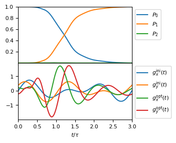
Notice the very fast convergence; this is one of the advantages of Krotov’s algorithm. The speed of convergence, and the quality of the maximum, will however depend on the value of \(\alpha\).

We now plot the results: in the top plot, the populations of the states as they evolve in time; in the bottom plot, the initial and optimized pulses.

pulses.pulse_collection_set_parameters(ft, x)
ts = np.linspace(0, T, ntsteps)
res = solvers.solve('rk4', H, ft, psi[0], ts)
ps = np.zeros([ntsteps, d])
for k in range(d):
    for j in range(ntsteps):
        ps[j, k] = qt.expect(psi[k]*psi[k].dag(), res[j])

plt.rcParams["font.size"] = "8"
plt.rcParams["figure.autolayout"] = False

fig, ax = plt.subplots(2, 1, figsize=(3, 3), sharex = True)
fig.subplots_adjust(hspace=0)

ax[0].plot(ts/tau, ps[:, 0], label = r"$P_0$")
ax[0].plot(ts/tau, ps[:, 1], label = r"$P_1$")
ax[0].plot(ts/tau, ps[:, 2], label = r"$P_2$")
#ax.set_xlabel(r"$t/\tau$")
ax[0].set_xlim(0, T/tau)
ax[0].set_ylim(0, 1)
ax[0].set_yticks([0.2, 0.4, 0.6, 0.8, 1.0])
ax[0].legend(bbox_to_anchor = (1.0, 1.0), loc = 'upper left')

ts = np.linspace(0, T, 400)

ax[1].plot(ts/tau, f0[0].fu(ts), label = r"$g_x^{\rm ini}(t)$")
ax[1].plot(ts/tau, f0[1].fu(ts), label = r"$g_y^{\rm ini}(t)$")
ax[1].plot(ts/tau, ft[0].fu(ts), label = r"$g_x^{\rm opt}(t)$")
ax[1].plot(ts/tau, ft[1].fu(ts), label = r"$g_y^{\rm opt}(t)$")
ax[1].set_xlabel(r"$t/\tau$")
ax[1].set_xlim(0, T/tau)
ax[1].legend(bbox_to_anchor = (1.0, 1.0), loc = 'upper left')

plt.show()

# This file is used by the testing script of the code.
with open("data", "w") as f:
    for i in data:
        f.write("{:.14e}\n".format(i))