4.5. Floquet optimization on a closed system
This tutorial demonstrates a Floquet optimization on a simple three-level quantum model of the Nitrogen-vancancy center in diamond. The goal is to find a periodic driving that modifies the Floquet pseudoenergies of the system, in such a way that a certain function of these pseudoenergies is maximized.
What we will do is to define a reference periodic driving, that leads to a set of reference pseudoenergies, and then do an optimization that attempts to find another periodic driving that leads to the same pseudoenergies (of course, the found optimal driving could be the same as the reference one, although in this case this is not what happens). In order to achieve this goal, we define a function of the pseudoenergies that measures the distance to the reference ones.
The model is defined by the three-level Hamiltonian:
\begin{eqnarray} H(u, t) &=& H_0 + V(u, t), \\ H_0 &=& -B_s S_z + N_z S_z^2 + N_{xy}(S_x^2-S_y^2), \\ \label{eq:tdpart} V(u, t) &=& - g_x(u, t) B_d S_x - g_y(u, t) B_d S_y. \end{eqnarray}
This model is taken from [Ikeda et al, Science Advances 6, eabb4019 (2020)]. \(S_x, S_y\) and \(S_z\) are the spin operators, whereas \(N_z\), \(N_{xy}\), \(B_s\), and \(B_d\) are constants. The shape of the real time-dependent control functions \(g_x\) and \(g_y\), dependent on the control parameters \(u\), is explained below.
[1]:
import os
import numpy as np
import qutip as qt
import nlopt
import matplotlib as mpl
import matplotlib.pyplot as plt
[2]:
import qocttools
import qocttools.pulses as pulses
import qocttools.qoct as qoct
import qocttools.hamiltonians as hamiltonians
import qocttools.floquet as floquet
import qocttools.target as target
It is good practice to print the precise version of the software that you are using.
[3]:
qocttools.about()
No git dir found
Running qocttools version 0.0.14
[4]:
data = []
Now, we build the static Hamiltonian \(H_0\) (stored into the Qobj object H0), and the two coupling operators \(V_1 = -B_d S_x\) and \(V_2 = -B_d S_y\) (stored into the Qobj objects V[0] and V[1]). The function system_definition in principle returns some Lindblad operators, but those are not used in this tutorial. The field-free eigenvalues are stored stored in the array e and the eigenfunctions in psi.
[5]:
Sx = qt.jmat(1, "x")
Sy = qt.jmat(1, "y")
Sz = qt.jmat(1, "z")
Bs = 0.3
Nz = 1.00
Nxy = 0.05
Bd = 0.1
omega = 1.00
gamma = 0.2
beta = 3.0
d = 3
dim = d**2
[6]:
def system_definition():
    H0 = -Bs * Sz + Nz * Sz**2 + Nxy * (Sx**2 - Sy**2)
    Vx = -Bd * Sx
    Vy = -Bd * Sy
    A = []
    e, psi = H0.eigenstates()
    for i in range(d):
        for j in range(d):
            if j == i:
                continue
            gammaij = gamma * np.exp(-beta*e[j]) / (np.exp(-beta*e[i])+np.exp(-beta*e[j]))
            A.append( np.sqrt(gammaij) * psi[j] * psi[i].dag())
    return H0, [Vx, Vy], A, e, psi

H0, V, A, e, psi = system_definition()
[7]:
print("Field-free eigenvalues = {}".format(e))
Field-free eigenvalues = [0. 0.69586187 1.30413813]
We must set a value for the period of the driving, and the corresponding frequency. That is of course problem dependent; for this tutorial we will arbitrarily use \(\omega = 3\). In this way, the Floquet-Brillouin zone is set to be \([-1.5, 1.5)\).
[8]:
omega = 3.0
T = (2.0*np.pi/omega)
print("The periodic driving frequency is {} eV.".format(omega))
print("The Floquet period is {} a.u".format(T))
The periodic driving frequency is 3.0 eV.
The Floquet period is 2.0943951023931953 a.u
We will first define some reference periodic driving: a circularly polarized field with a single frequency, omega. But we will first do a zero-field calculation, setting the amplitude to zero, which should yield some pseudoenergies that are equal to the system eigenvalues. In order to compute the pseudoenergies, we will use the epsilon() function from the floquet module.
[9]:
a0 = 0.0

def Axref(t, args):
    return a0 * np.sin(omega * t)

def Ayref(t, args):
    return a0 * np.cos(omega * t)
This is one way to specify a time-dependent Hamiltonian when using qutip (see the qutip documentation for details). This is the format that the function epsilon() expects.
[10]:
H = [H0, [V[0], Axref], [V[1], Ayref]]
[11]:
epsilon0 = floquet.epsilon(H, T)
print("Field-free Floquet pseudoenergies = {}".format(epsilon0))
Field-free Floquet pseudoenergies = [-0. 0.69586188 1.30413865]
As it can be seen, the pseudoenergies are equal to the energies. Let us now redo the calculation, but using a non-zero amplitude.
[12]:
a0 = 5.0
[13]:
epsilon_ref = floquet.epsilon(H, T)
print("Reference Floquet pseudoenergies = {}".format(epsilon_ref))
print("Field-free Floquet pseudoenergies = {}".format(epsilon0))
print("Diff with the field-free eigenvalues = {}".format(epsilon_ref-epsilon0))
Reference Floquet pseudoenergies = [0.03783496 0.7288814  1.23328367]
Field-free Floquet pseudoenergies = [-0.          0.69586188  1.30413865]
Diff with the field-free eigenvalues = [ 0.03783496  0.03301952 -0.07085499]
The pseudoenergies in epsilon_ref are now the target pseudoenergies.
We will now define the parametrized pulses (Fourier series, in this example), whose parameters will be used for the optimization. In the code below, we have the option of reading the pulses from a file (if the pulses have been stored in a file in a previous run), generating a random pulse, or using some predefined values for the parameters. The last thing is what we do in the tutorial – although, in fact, the values were previously randomly generated; we hardcode them here in order to ensure that the tutorial always produces the same numbers.
[14]:
times = np.linspace(0, T, 100)
maxamp = a0 * np.sqrt(T) / 2
[15]:
read_initial_guess_from_disk = False
[16]:
if not read_initial_guess_from_disk:

    M = 5
    random_initial_pulse = False

    if random_initial_pulse:
        random_bound = 1.0 * maxamp
        u1 = np.zeros(2*M+1)
        u1[1:] = np.random.uniform(low = -1.0, high = 1.0, size = 2*M)
        u1[1:] = random_bound * u1[1:]
        u2 = np.zeros(2*M+1)
        u2[1:] = np.random.uniform(low = -1.0, high = 1.0, size = 2*M)
        u2[1:] = random_bound * u2[1:]
    else:
        # These numbers were random-generated. We hard-code them here, to ensure the
        # exact reproducibility of the tutorial results.
        u1 = np.array([0.0, 0.3781672550042017, 3.337578192688232,
                       0.39792661221249986, 2.640586714801746,
                       1.275967487033285, -1.0266663277960986,
                       1.690341853324815, -2.7232255567616743,
                       -0.20406687253848577, 1.020998297311514])
        u2 = np.array([0.0, -0.8765685785388411, 3.059796305834288,
                       -1.3956891274241654, 2.931174340624856,
                       -2.03904569878065, -1.6616521056176727,
                       3.3729352354374806, -1.0565599367266927,
                       2.7168660074286004, -0.229243896077151])

    Ax0 = pulses.pulse("fourier", T, u = u1)
    Ay0 = pulses.pulse("fourier", T, u = u2)
    Axopt = pulses.pulse("fourier", T, u = u1)
    Ayopt = pulses.pulse("fourier", T, u = u2)
    Ax0.print('Ax0')
    Ay0.print('Ay0')
else:
    Ax0 = pulses.read_pulse('Ax0')
    Ay0 = pulses.read_pulse('Ay0')
    Axopt = pulses.read_pulse('Ax0')
    Ayopt = pulses.read_pulse('Ay0')
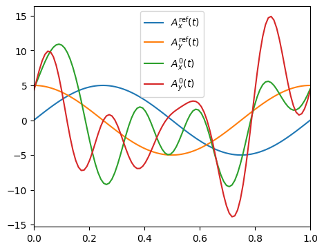
Let us make a plot of the initial-guess for the drivings:
[17]:
fig = plt.figure(figsize=(5,4))
ax = fig.add_axes([0.15, 0.15, 0.8, 0.8])

times = np.linspace(0, T, 100)

ax.plot(times/T, Axref(times, None), label = r"$A^{\rm ref}_x(t)$")
ax.plot(times/T, Ayref(times, None), label = r"$A^{\rm ref}_y(t)$")

ax.plot(times/T, Ax0.fu(times), label = r"$A^{\rm 0}_x(t)$")
ax.plot(times/T, Ay0.fu(times), label = r"$A^{\rm 0}_y(t)$")

ax.legend()
ax.set_xlim(left = 0, right = 1)

plt.show()
The variable u0 holds all the parameters, from both pulses.
[18]:
u0 = pulses.pulse_collection_get_parameters([Ax0, Ay0])
We now need to create a hamiltonian object.
[19]:
H = hamiltonians.hamiltonian(H0, V)
Let us now compute the pseudo-energies with the parameters of the initial-guess pulses:
[20]:
u = u0.copy()
[21]:
epsilon_ig = floquet.epsilon3(H, [Ax0, Ay0], u, T)
print("Initial-guess Floquet pseudoenergies = {}".format(epsilon_ig))
print("Reference Floquet pseudoenergies = {}".format(epsilon_ref))
print("Diff = {}".format(epsilon_ig-epsilon_ref))
Initial-guess Floquet pseudoenergies = [0.03532867 0.70549711 1.25917425]
Reference Floquet pseudoenergies = [0.03783496 0.7288814  1.23328367]
Diff = [-0.00250629 -0.02338429  0.02589059]
Next step is the definition of the target function \(f(\varepsilon)\), and its gradient. This is done in the following cell. The definition is: \begin{equation} f(\varepsilon) = -\sum_\alpha (\varepsilon_\alpha - \varepsilon^{\rm ref}_\alpha)^2 \end{equation} The maximum of this function is achieved when \(\varepsilon = \varepsilon^{\rm ref}\), and then \(f(\varepsilon)=0\).
[22]:
targeteps = epsilon_ref.reshape(1, 3)

def f(eps):
    cte = 1.0
    fval = 0.0
    nkpoints = eps.shape[0]
    targete = targeteps
    dim = eps.shape[1]
    fval = 0.0
    for k in range(nkpoints):
        for alpha in range(dim):
            fval = fval - cte * (eps[k, alpha] - targete[k, alpha])**2
    return fval

def dfdepsilon(eps):
    cte = 1.0
    nkpoints = eps.shape[0]
    targete = targeteps
    dim = eps.shape[1]
    dfval = np.zeros((nkpoints, dim))
    for k in range(nkpoints):
        for alpha in range(dim):
            dfval[k, alpha] = - 2.0 * cte * (eps[k, alpha]-targete[k, alpha])
    return dfval
4.5.1. Computation based on perturbation theory in Floquet-Hilbert space
First, let us do the optimization using the expression from the gradient based on perturbation theory in Floquet-Hilbert space, as described here
[23]:
u = u0.copy()
pulses.pulse_collection_set_parameters([Axopt, Ayopt], u)
We define the target object. Note that we need to tell qocttools about function \(f\) and its gradient, defined above.
[24]:
tg = target.Target('floquet', targeteps = targeteps,
                   T = T, fepsilon = f, dfdepsilon = dfdepsilon)
Now, the Qoct object.
[25]:
U0set = [qt.qeye(3)]
opt = qoct.Qoct(H, T, times.shape[0], tg, [Axopt, Ayopt], U0set, floquet_mode = 'pt')
Let us look at the value of the target function with the initial-guess parameters:
[26]:
print("G(u) = {} (initial guess)".format(opt.gfunc(u)))
G(u) = -0.0012234288619094999 (initial guess)
We now do the optimization.
[27]:
check_gradient = True
if check_gradient:
    derqoct, dernum, error, elapsed_time = opt.check_grad(u)
    print("QOCT calculation: \t{}".format(derqoct))
    print("Ridders calculation: \t{} +- {}".format(dernum, error))

optimize = True

if optimize:
    x, optval, res = opt.maximize(maxeval = 100,
                                  verbose = True,
                                  algorithm = nlopt.LD_SLSQP,
                                  upper_bounds = 1 * np.abs(maxamp * np.ones_like(u)),
                                  lower_bounds = -1 * np.abs(maxamp * np.ones_like(u)))
    uopt = pulses.pulse_collection_get_parameters([Axopt, Ayopt])
    print(opt.gfunc(uopt))
    epsilon_opt1 = floquet.epsilon3(H, [Axopt, Ayopt], uopt, T)
    print("Optimized Floquet pseudoenergies = {}".format(epsilon_opt1))
    print("Reference Floquet pseudoenergies = {}".format(epsilon_ref))
    print("Diff = {}".format(epsilon_opt1-epsilon_ref))
QOCT calculation:       -0.0011906265027648202
Ridders calculation:    -0.0011906296479533565 +- 1.1073355509448601e-09
0 -0.001223 (0.097985 s)
1 -0.001220 (0.085048 s)
2 -0.001201 (0.092715 s)
3 -0.001112 (0.091922 s)
4 -0.000727 (0.093350 s)
5 -0.000096 (0.086242 s)
6 -0.000095 (0.090300 s)
7 -0.000090 (0.089479 s)
8 -0.000074 (0.090592 s)
9 -0.000068 (0.091312 s)
10 -0.000067 (0.091188 s)
11 -0.000061 (0.096273 s)
12 -0.000036 (0.093577 s)
13 -0.000006 (0.086093 s)
14 -0.000002 (0.090773 s)
15 -0.000000 (0.090215 s)
16 -0.000000 (0.089643 s)
Successfull termination with result code = 3
("Function tolerance reached")
-2.8594517503162082e-08
Optimized Floquet pseudoenergies = [0.03791892 0.72874449 1.2333366 ]
Reference Floquet pseudoenergies = [0.03783496 0.7288814  1.23328367]
Diff = [ 8.39560069e-05 -1.36908104e-04  5.29346530e-05]
The optimization is successfull (we reach the absolute maximum value of zero). How does the optimal driving compare with the refernce one? We can look at both in the following plot:
[28]:
fig = plt.figure(figsize=(5,4))
ax = fig.add_axes([0.15, 0.15, 0.8, 0.8])

times = np.linspace(0, T, 100)

ax.plot(times/T, Axref(times, None), label = r"$A^{\rm ref}_x(t)$")
ax.plot(times/T, Ayref(times, None), label = r"$A^{\rm ref}_y(t)$")

ax.plot(times/T, Axopt.fu(times), label = r"$A^{\rm opt}_x(t)$")
ax.plot(times/T, Ayopt.fu(times), label = r"$A^{\rm opt}_y(t)$")

ax.legend()
ax.set_xlim(left = 0, right = 1)

plt.show()
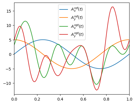
Surprisingly (or perhaps not so much), the fields are different. Different drivings can produce the same pseudoenergies.
4.5.2. Computation based on a QOCT formula
Now, let us do the same optimization, but using the expression from the gradient based on QOCT, as described here
[29]:
u = u0.copy()
pulses.pulse_collection_set_parameters([Axopt, Ayopt], u)
We define the target object. Note that we need to tell qocttools about function \(f\) and its gradient, defined above.
[30]:
tg = target.Target('floquet', targeteps = targeteps,
                   T = T, fepsilon = f, dfdepsilon = dfdepsilon)
Now, the Qoct object.
[31]:
opt = qoct.Qoct(H, T, times.shape[0], tg, [Axopt, Ayopt], U0set, floquet_mode = 'qoct')
print("G(u) = {} (initial guess)".format(opt.gfunc(u)))
G(u) = -0.0012234331435382868 (initial guess)
And finally, the optimization
[32]:
check_gradient = True
if check_gradient:
    #u = pulses.pulse_collection_get_parameters([Axopt, Ayopt])
    derqoct, dernum, error, elapsed_time = opt.check_grad(u)
    print("QOCT calculation: \t{}".format(derqoct))
    print("Ridders calculation: \t{} +- {}".format(dernum, error))
    data.append(derqoct)
QOCT calculation:       -0.0011906311737541137
Ridders calculation:    -0.0011906290761807378 +- 2.6183482465524932e-15
[33]:
optimize = True

if optimize:
    x, optval, res = opt.maximize(maxeval = 100,
                                  verbose = True,
                                  #tolerance = -1.0,
                                  #algorithm = nlopt.LD_MMA,
                                  algorithm = nlopt.LD_SLSQP,
                                  #algorithm = nlopt.LN_BOBYQA,
                                  #algorithm = nlopt.GD_STOGO,
                                  #algorithm = nlopt.LD_LBFGS,
                                  upper_bounds = 1 * np.abs(maxamp * np.ones_like(u)),
                                  lower_bounds = -1 * np.abs(maxamp * np.ones_like(u)))
    uopt = pulses.pulse_collection_get_parameters([Axopt, Ayopt])
    print(opt.gfunc(uopt))
    epsilon_opt2 = floquet.epsilon3(H, [Axopt, Ayopt], uopt, T)
    print("Optimized Floquet pseudoenergies = {}".format(epsilon_opt2))
    print("Reference Floquet pseudoenergies = {}".format(epsilon_ref))
    print("Diff = {}".format(epsilon_opt2-epsilon_ref))
    data.append(optval)
0 -0.001223 (0.036484 s)
1 -0.001220 (0.035280 s)
2 -0.001201 (0.035848 s)
3 -0.001112 (0.035461 s)
4 -0.000727 (0.035374 s)
5 -0.000096 (0.035692 s)
6 -0.000095 (0.037385 s)
7 -0.000090 (0.038666 s)
8 -0.000074 (0.035397 s)
9 -0.000068 (0.034065 s)
10 -0.000067 (0.035340 s)
11 -0.000061 (0.035501 s)
12 -0.000036 (0.038216 s)
13 -0.000006 (0.035648 s)
14 -0.000002 (0.037761 s)
15 -0.000000 (0.035960 s)
16 -0.000000 (0.033571 s)
Successfull termination with result code = 3
("Function tolerance reached")
-2.8599392189165148e-08
Optimized Floquet pseudoenergies = [0.03791895 0.72874453 1.23333653]
Reference Floquet pseudoenergies = [0.03783496 0.7288814  1.23328367]
Diff = [ 8.39888103e-05 -1.36866988e-04  5.28607314e-05]
Since, after all, we are just using two alternative methods to compute the same gradient, we get the same result.
[34]:
# This file is used by the testing script of the code.
with open("data", "w") as f:
    for i in data:
        f.write("{:.14e}\n".format(i))