4.4. Optimization for an open system

This tutorial demonstrates a basic optimization of a simple three-level quantum model of the Nitrogen-vancancy center in diamond. It is treated as an open system (using the time-dependent Lindblad equation), subject to some dissipative terms.

The goal is to find a pulse that attempts to maintain the system in the first excited state, as much as possible, fighting the dissipation induced the environment that would otherwise drive the system towards the thermal state. In other words, we start the simulation from the first excited state, and try to find that pulse which, at the end of the simulation time \(T\), produces the highest possible population of that same state.

The model is defined by the three-level Hamiltonian:

\begin{eqnarray} H(u, t) &=& H_0 + V(u, t), \\ H_0 &=& -B_s S_z + N_z S_z^2 + N_{xy}(S_x^2-S_y^2), \\ \label{eq:tdpart} V(u, t) &=& - g_x(u, t) B_d S_x - g_y(u, t) B_d S_y. \end{eqnarray}

This model is taken from [Ikeda et al, Science Advances 6, eabb4019 (2020)]. \(S_x, S_y\) and \(S_z\) are the spin operators, whereas \(N_z\), \(N_{xy}\), \(B_s\), and \(B_d\) are constants. The shape of the real time-dependent control functions \(g_x\) and \(g_y\) is explained below.

The system is governed by Lindblad’s equation:

\begin{align} \dot{\rho}(t) = -i\left[H(u, t), \rho(t)\right] + \sum_{ij} \gamma_{ij} \left( V_{ij}\rho(t)V^\dagger_{ij} - \frac{1}{2} \lbrace V_{ij}^\dagger V_{ij}, \rho(t) \rbrace\right)\,. \label{eq:lindblad0-eq} \end{align}

The transition operators are \(V_{ij} = \vert E_i\rangle\langle E_j\vert\), and the dissipative constants are \(\gamma_{ij} = \gamma e^{-\beta E_i} / (e^{-\beta E_i}+e^{-\beta E_j})\) and \(\gamma_{ii}=0\), where \(\beta = 1/(k_{\rm B}T)\) is the inverse of the temperature, and \(\gamma\) is a rate constant. Notice that this dissipation model ensures the detailed balance condition, \(\gamma_{ij}e^{-\beta E_j} = \gamma_{ji}e^{-\beta E_i}\).

import numpy as np
import matplotlib
from copy import deepcopy
import matplotlib.pyplot as plt
import qutip as qt
import nlopt

import qocttools
import qocttools.hamiltonians as hamiltonians
import qocttools.target as target
import qocttools.pulses as pulses
import qocttools.qoct as qoct
import qocttools.solvers as solvers

It is good practice to print the precise version of the software that you are using.

qocttools.about()

No git dir found

Running qocttools version 0.0.14

Now, we build the static Hamiltonian \(H_0\) (stored into the Qobj object H0), and the two coupling operators \(V_1 = -B_d S_x\) and \(V_2 = -B_d S_y\) (stored into the Qobj objects V[0] and V[1]). The function system_definition also returns some Lindblad operators into the A list, as defined above. The field-free eigenvalues are stored stored in the array e and the eigenfunctions in psi.

Sx = qt.jmat(1, "x")
Sy = qt.jmat(1, "y")
Sz = qt.jmat(1, "z")
Bs = 0.3
Nz = 1.00
Nxy = 0.05
Bd = 0.1
omega = 1.00
gamma = 0.01
beta = 3.0
d = 3
dim = d**2

def system_definition():
    H0 = -Bs * Sz + Nz * Sz**2 + Nxy * (Sx**2 - Sy**2)
    Vx = -Bd * Sx
    Vy = -Bd * Sy
    A = []
    e, psi = H0.eigenstates()
    for i in range(d):
        for j in range(d):
            if j == i:
                continue
            gammaij = gamma * np.exp(-beta*e[j]) / (np.exp(-beta*e[i])+np.exp(-beta*e[j]))
            A.append( np.sqrt(gammaij) * psi[j] * psi[i].dag())
    return H0, [Vx, Vy], A, e, psi

H0, V, A, e, psi = system_definition()

print("Field-free eigenvalues = {}".format(e))

Field-free eigenvalues = [0.         0.69586187 1.30413813]

The first step is to create the an object of hamiltonian class:

H = hamiltonians.hamiltonian(H0, V, A)

For later use, let us compute the equilibrium thermal state, \(\rho_\beta = \frac{e^{-\beta H_0}}{{\rm Tr}e^{-\beta H_0}}\)

rhothermal = (-beta * H0).expm()
rhothermal = rhothermal / rhothermal.tr()

Let us define a relevant frequency, characteristic of the system, that gives us an idea of the energies and time scales. omega will be given by the energy difference between the ground and first excited state. Correspondingly, we can define a relevant period, corresponding to that frequency

omega = e[1]-e[0]
tau = 2.0*np.pi/omega

Now we consider the total propagation time. To make the transition easier, it is useful to make sure that the total propagation time includes several time the relevant period tau. In this case, we will make it ten times larger. This also defines a “fundamental frequency”, \(\omega_0 = 2\pi/T\).

T = 10 * tau
omega0 = 2.0*np.pi/T
print("omega0 = {:.4f}".format(omega0))

omega0 = 0.0696

Now we create the Target object. In this case, it is an “expectationvalue” type, since what we want to do is to maximize the expectation value of \(O = \vert\phi_1\rangle \langle\phi_1\vert\), i.e. the population of the first excited state.

O = psi[1] * psi[1].dag()
tg = target.Target("expectationvalue", operator = O, T = T)

Now, we must create the pulse objects, i.e. the control functions. In this case, we have two perturbation operators, and we need two control functions. In this example, we will choose a Fourier-series parametrization for both control functions.

A Fourier series must be cutoff at some maximum frequency \(M\omega_0\). We will set \(M=15\), which ensures that the relevant frequency \(\omega\) is lower than the maximum frequency. Then we must give initial-guess values to the amplitudes of the Fourier series (which are the control parameters). There are \(2M+1\) parameteres in each Fourier series (\(M\) for the cosines, \(M\) for the sines, and 1 for the zero-frequency term). We will simply set some of the parameters to some \(\kappa\) value, and zero for the rest of them.

A better alternative would be to use random values, but in order to make sure that the tutorial always produces the same result, we will not use that option here.

M = 15
kappa = 0.1

u1 = np.zeros(2*M+1)
u2 = np.zeros(2*M+1)
u1[3] = kappa
u2[4] = kappa

# The following code sets random numbers for the control parameters
#a = -bound
#b = bound
#u1 = (b-a) * np.random.rand(2*M+1) + a
#u2 = (b-a) * np.random.rand(2*M+1) + a

We place the pulse objects into a list f.

f = []
f.append(pulses.pulse("fourier", T, u = u1))
f.append(pulses.pulse("fourier", T, u = u2))
f0 = deepcopy(f)

We also define a couple of zero pulses, so that we can propagate the free system to make comparisons.

fnull = []
fnull.append(pulses.pulse("fourier", T, u = np.zeros_like(u1)))
fnull.append(pulses.pulse("fourier", T, u = np.zeros_like(u2)))

u0 will hold all the control parameters (the parameters of all the pulses together). unull are the parameters of the zero pulses.

u0 = pulses.pulse_collection_get_parameters(f)
unull = pulses.pulse_collection_get_parameters(fnull)

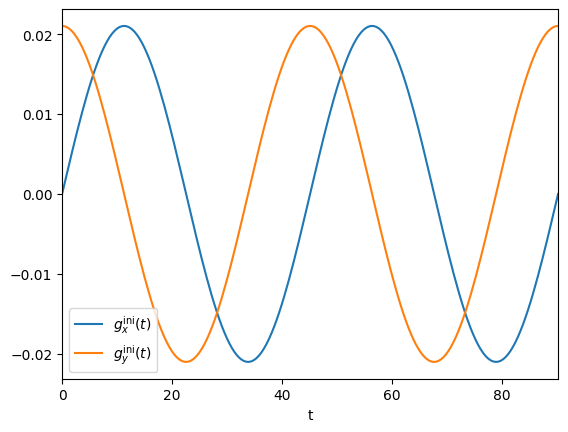
Let us plot to see how the pulses look like.

fig, ax = plt.subplots()

ts = np.linspace(0, T, 200)
ax.plot(ts, f0[0].fu(ts), label = r"$g_x^{\rm ini}(t)$")
ax.plot(ts, f0[1].fu(ts), label = r"$g_y^{\rm ini}(t)$")
ax.set_xlabel("t")
ax.set_xlim(0, T)
ax.legend()

plt.show()

We now build the main object, of class Qoct. Along with the Hamiltonian H, the target tg, and the set of control functions f, we need to pass the initial state, in our case the first excited state psi[1]. Also, ntsteps, which is the number of time steps used to discretize the time interval for the numerical integration. The higher, the more precise the calculations will be, but they will also be slower.

rho0 = psi[1] * psi[1].dag()

ntsteps = 150
opt = qoct.Qoct(H, T, ntsteps, tg, f, rho0)

Let us see what the initial pulse does: we will propagate the system using the initial guess pulses, and we will plot the populations of each state as a function of time. But first, we will propagate the system with no external fields, so that we can compare.

In order to the system propagation, we will use the solve() function and, in this case, the cfmagnus4 method (see the documentation of the solve() function to learn about the propagation methods used by qocttools).

ts = np.linspace(0, T, ntsteps)
res = solvers.solve('cfmagnus4', H, fnull, rho0, ts)
ps = np.zeros([ntsteps, d+1])
for j in range(ntsteps):
    for k in range(d):
        ps[j, k] = qt.expect(psi[k] * psi[k].dag(), res[j])
    ps[j, d] = qt.fidelity(rhothermal, res[j])

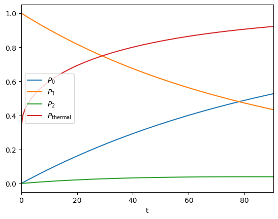
We plot now the populations of the three states, as the system decays from the first state. We also plot the fidelity of the evolving state with respect to the thermal state, to which it would eventually converge.

fig, ax = plt.subplots()
ax.plot(ts, ps[:, 0], label = r"$P_0$")
ax.plot(ts, ps[:, 1], label = r"$P_1$")
ax.plot(ts, ps[:, 2], label = r"$P_2$")
ax.plot(ts, ps[:, 3], label = r"$P_{\rm thermal}$")
ax.set_xlabel("t")
ax.set_xlim(0, T)
ax.legend()
plt.show()

We now propagate the sytemm in the presence of the initial guess pulse.

ts = np.linspace(0, T, ntsteps)
res = solvers.solve('cfmagnus4', H, f, rho0, ts)
ps = np.zeros([ntsteps, d+1])
for j in range(ntsteps):
    for k in range(d):
        ps[j, k] = qt.expect(psi[k] * psi[k].dag(), res[j])
    ps[j, d] = qt.fidelity(rhothermal, res[j])

fig, ax = plt.subplots()
ax.plot(ts, ps[:, 0], label = r"$P_0$")
ax.plot(ts, ps[:, 1], label = r"$P_1$")
ax.plot(ts, ps[:, 2], label = r"$P_2$")
ax.plot(ts, ps[:, 3], label = r"$P_{\rm thermal}$")
ax.set_xlabel("t")
ax.set_xlim(0, T)
ax.legend()
plt.show()

As one can see, the initial guess pulse does not do much: the population of the excited state decays in a similar way with respect to the zero-field case.

Before launching the optimization, one can check that the gradient is computed correctly. We can use for that purpose the check_grad() method of the Qoct class. It computes the gradient using the QOCT formula, and using finite differences. Both numbers should match if everything is OK. Uncomment the following lines if you want to do that check.

#derqoct, dernum, error = opt.check_grad(u0)
#print(derqoct, dernum, error)

Finally, we launch the maximization calculation, using the maximize() method. Note that we have added bounds on the parameters, using the upper_bounds and lower_bounds arguments. In this way, we force the algorithm to find a solution that will be contained within thouse bounds.

x, optval, result = opt.maximize(maxeval = 40,
                                 stopval = 0.99,
                                 verbose = True,
                                 algorithm = nlopt.LD_SLSQP,
                                 upper_bounds = 5.0 * kappa * np.ones_like(u0),
                                 lower_bounds = -5.0 * kappa * np.ones_like(u0))

0 0.433616 (0.371710 s)
1 0.433618 (0.604339 s)
2 0.433633 (0.457388 s)
3 0.434454 (0.609400 s)
4 0.502428 (0.533273 s)
5 0.529862 (0.588562 s)
6 0.565732 (0.607115 s)
7 0.599705 (0.370468 s)
8 0.611566 (0.505498 s)
9 0.631113 (0.606469 s)
10 0.646542 (0.535597 s)
11 0.654159 (0.606036 s)
12 0.658493 (0.468646 s)
13 0.662235 (0.524256 s)
14 0.663524 (0.607564 s)
15 0.666192 (0.465120 s)
16 0.666966 (0.605414 s)
17 0.668105 (0.445905 s)
18 0.670814 (0.607837 s)
19 0.671444 (0.369509 s)
20 0.672423 (0.448549 s)
21 0.673545 (0.601251 s)
22 0.675244 (0.610517 s)
23 0.677684 (0.502680 s)
24 0.686869 (0.608828 s)
25 0.690606 (0.469898 s)
26 0.705371 (0.388143 s)
27 0.726475 (0.608531 s)
28 0.731304 (0.467993 s)
29 0.747467 (0.602077 s)
30 0.751716 (0.608775 s)
31 0.758222 (0.411369 s)
32 0.763166 (0.607361 s)
33 0.765432 (0.404814 s)
34 0.767419 (0.606729 s)
35 0.769337 (0.374678 s)
36 0.771987 (0.608046 s)
37 0.772874 (0.469043 s)
38 0.773759 (0.606305 s)
39 0.774351 (0.467950 s)
Successfull termination with result code = 5
("Maximum evaluations reached")

Let us now propagate the sytem in the presence of the optimal pulse found by the algorithm, and see how it does.

ts = np.linspace(0, T, ntsteps)
res = solvers.solve('cfmagnus4', H, f, rho0, ts)
ps = np.zeros([ntsteps, d])
for k in range(d):
    for j in range(ntsteps):
        ps[j, k] = qt.expect(psi[k]*psi[k].dag(), res[j]).real

fig, ax = plt.subplots()
ax.plot(ts, ps[:, 0], label = r"$P_0$")
ax.plot(ts, ps[:, 1], label = r"$P_1$")
ax.plot(ts, ps[:, 2], label = r"$P_2$")
ax.set_xlabel("t")
ax.set_xlim(0, T)
ax.legend()
plt.show()

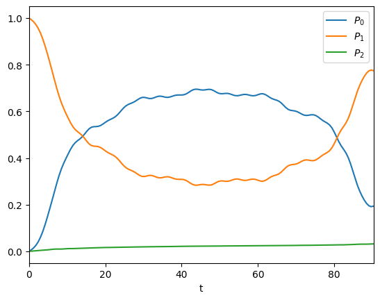
As one can see, the population of the first excited state at the end of the propagation is higher now.

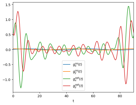
Finally, we compare now in a plot the initial guess versus the optimized pulse.

fig, ax = plt.subplots()

ts = np.linspace(0, T, 200)
ax.plot(ts, f0[0].fu(ts), label = r"$g_x^{\rm ini}(t)$")
ax.plot(ts, f0[1].fu(ts), label = r"$g_y^{\rm ini}(t)$")
ax.plot(ts, f[0].fu(ts), label = r"$g_x^{\rm opt}(t)$")
ax.plot(ts, f[1].fu(ts), label = r"$g_y^{\rm opt}(t)$")
ax.set_xlabel("t")
ax.set_xlim(0, T)
ax.legend()

plt.show()